Perceptrons
variationalform https://variationalform.github.io/
Just Enough: progress at pace
https://variationalform.github.io/
https://github.com/variationalform
Simon Shaw https://www.brunel.ac.uk/people/simon-shaw.
|
|
This work is licensed under CC BY-SA 4.0 (Attribution-ShareAlike 4.0 International) Visit http://creativecommons.org/licenses/by-sa/4.0/ to see the terms. |
| This document uses python |

|
and also makes use of LaTeX |

|
in Markdown |
|
What this is about:
The perceptron
- weighted inputs
- activation thresholds and outputs
- decision boundaries
- multi-layer perceptrons
- feed-forward artificial neural network
As usual our emphasis will be on doing rather than proving: just enough: progress at pace
Assigned Reading
For this material you are recommended Chapter 3 of [UDL], then Chapter 3 of [NND], and Chapter 6 of [MLFCES],
- UDL: Understanding Deep Learning, by Simon J.D. Prince. PDF draft available here: https://udlbook.github.io/udlbook/
- NND: Neural Network Design by Martin T. Hagan, Howard B. Demuth, Mark Hudson Beale, Orlando De Jesús. https://hagan.okstate.edu/nnd.html and https://hagan.okstate.edu/NNDesign.pdf
- MLFCES: Machine Learning: A First Course for Engineers and Scientists, by Andreas Lindholm, Niklas Wahlström, Fredrik Lindsten, Thomas B. Schön. Cambridge University Press. http://smlbook.org.
These can be accessed legally and without cost.
There are also these useful references for coding:
- PT:
python: https://docs.python.org/3/tutorial - NP:
numpy: https://numpy.org/doc/stable/user/quickstart.html - MPL:
matplotlib: https://matplotlib.org
Context
In the last two sessions we moved from classification to regression and then we moved back to classification again.
We have focussed on cases where the data is linearly separable. This important property allowed us to use logistic regression and support vector machines to construct linear decision boundaries.
In this session we will continue to work with linear decision boundaries and investigate the perceptron and feed forward neural networks.
The main purpose of this session is to get insight into how perceptrons can carve up high dimensional space with hyperplanes, thus creating many compartments within which data classes can be isolated. This will set us up nicely for our study of deep neural networks.
The Percepton - and a Shallow Neural Network
A perceptron is a computing unit that accepts a vector of numerical inputs, $\boldsymbol{x}$, and forms a linear combination of them using a vector of weights, $\boldsymbol{W}$. A numerical bias, $b$, may then be added to form a real number.
This real number is then thresholded with an activation function. This activation function seeks to determine how significant its input signal is and either kills it or passes it some form of it through.
The whole system is an attempt to (very crudely) mimic the neuronal connections in the brain.
Chapters 2 and 3 of [UDL, Chapter 3] https://udlbook.github.io/udlbook/ are useful background reading, but what we do here is self-contained.
Here it is - schematically. The input vector $\boldsymbol{x}=(x_1,x_2,x_3)^T$, and weights, $\boldsymbol{W}=(w_1,w_2,w_3)^T$, are linearly combined. An optional bias, $b$, is added and the result, $n$ is fed into an activation function, $\sigma\colon\mathbb{R}\to\mathbb{R}$ to produce the output $y$.
$$ \begin{array}{lr} \begin{array}{ll} n & = w_1 x_1 + w_2 x_2 + w_3 x_3 + b, \\ & = \boldsymbol{W}^T\boldsymbol{x} + b, \\ y & = \sigma(n). \end{array} & \qquad\qquad \begin{array}{rlcll} x_1 & \boldsymbol{w}& & &\\ & \searrow & & \sigma(n) &\\ x_2 & \rightarrow & n\!\!\!\!\!\bigcirc & \longrightarrow & y \\ & \nearrow & \uparrow & & \\ x_3 & & b & & \\ & & & & \\ \end{array} \end{array} $$Compactly: $y = \sigma(\boldsymbol{W}^T\boldsymbol{x} + b)$. Let's see why this is so useful - it really comes down the the activation function. Without that this isn't such a big deal.
The Heaviside Unit Step function
This is defined as follows:
$$ \mathcal{H}(x) = \left\{\begin{array}{ll} 1 &\text{if } x > 0; \\ x_2 &\text{if } x = 0; \\ 0 &\text{if } x < 0. \end{array}\right. $$It represents a switch being thrown as the input increases through zero,
with the output signal moving from zero to one. The value $x_2$ at the
discontinuity is usually arbitrary. We have included it because numpy
allows it with this syntax:
np.heaviside(x,x2)We will usually take $x_2=0$. For details see here: https://numpy.org/doc/stable/reference/generated/numpy.heaviside.html
The Heaviside function can be used as an activation function - let's see it.
import matplotlib.pyplot as plt
import numpy as np
import numpy.matlib  # a new one, needed below for repmat
x_vals = np.arange(-20, 20.1, 0.1)
y_vals_1 = np.heaviside(x_vals, 0)
y_vals_2 = np.heaviside(x_vals - 5, 0)
y_vals_3 = 2*np.heaviside(x_vals + 8, 0)
plt.figure(figsize=(10,4)); plt.gca().set_aspect(10)
plt.plot(x_vals, y_vals_1, color='blue', label='H(x)')
plt.plot(x_vals, y_vals_2, color='red', label='H(x-5)')
plt.plot(x_vals, y_vals_3, color='green', label='2H(x+8)')
plt.xlabel('x'); plt.ylabel('Heaviside');
plt.legend()
plt.show()
NOTE: the vertical lines are an artefact of the plotting - they aren't part of the function's graph.
A simple feed forward neural net
Let's use this concrete example: two inputs $\boldsymbol{x}=(x_1,x_2)^T$, with weights, $\boldsymbol{W}=(w_1,w_2)^T=(3,2)^T$ and optional bias, $b=-1$. The activation function is the Heaviside function.
This gives the output,
$$ y = \mathcal{H}(n) \quad\text{ for }\quad n = \boldsymbol{W}^T\boldsymbol{x}+b = 3 x_1 + 2 x_2 - 1. $$Hence,
$$ y = \left\{\begin{array}{ll} 1 &\text{if } n > 0; \\ 0 &\text{if } n \le 0, \end{array}\right. \qquad\Longrightarrow\qquad y = \left\{\begin{array}{ll} 1 &\text{if } 3 x_1 + 2 x_2 - 1 > 0; \\ 0 &\text{if } 3 x_1 + 2 x_2 - 1 \le 0. \end{array}\right. $$This can be a binary classifier. Can you see why?
We have just seen that with the given weights and bias,
$$ y = \mathcal{H}(n)\text{ for } n = \boldsymbol{W}^T\boldsymbol{x}+b = 3 x_1 + 2 x_2 - 1 \ \Rightarrow\ y = \left\{\begin{array}{ll} 1 &\text{if } 3 x_1 + 2 x_2 - 1 > 0; \\ 0 &\text{if } 3 x_1 + 2 x_2 - 1 \le 0. \end{array}\right. $$In this $3 x_1 + 2 x_2 - 1 = 0$ represents a straight line in the $(x_1,x_2)$ plane. In the usual form of $y=mx+c$, this line has equation $x_2 = (1-3x_1)/2$. That is: gradient $-3/2$, and intercept $1/2$.
A point $(x_1,x_2)=(a,b)$ above this line has $3 x_1 + 2 x_2 - 1 > 0$ while a point on or below the line has $3 x_1 + 2 x_2 - 1 \le 0$.
Therefore - this line could be a decision boundary. Any other line could also, we would just need different choices for the weights and bias.
Let's set this up and do some calculations with $(x_1,x_2)=(3,1)$ and $(x_1,x_2)=(-2,-1)$.
$y = \mathcal{H}(n)$ for $\displaystyle n=(3,2){x_1 \choose x_2}-1$...
# set up our column vector of weights, and the bias
W = np.array([[3,2]]).T
b = -1
# find y for input x = (3,1)
X = np.array([[3,1]]).T
y = np.heaviside(W.T@X+b,0)
print('For input x = ( 3, 1), y = ', y)
# find y for input x = (-2,-1)
X = np.array([[-2,-1]]).T
y = np.heaviside(W.T@X+b,0)
print('For input x = (-2,-1), y = ', y)
For input x = ( 3, 1), y =  [[1.]]
For input x = (-2,-1), y =  [[0.]]
We can also illustrate this graphically. We plot the line and then the two input points
x_vals = np.arange(-5, 5.1)
y_vals = (1-3*x_vals)/2
plt.plot(x_vals, y_vals, color='black', label='decision boundary')
plt.plot( 3, 1, 'x', color='blue',label='(x1,x2)=( 3, 1)')
plt.plot(-2,-1, 'x', color='red', label='(x1,x2)=(-2,-1)')
plt.xlabel('x_1'); plt.ylabel('x_2');
plt.annotate('above', [ 0, 3], color='blue')
plt.annotate('below', [-2,-4], color='red')
plt.legend();  # the semi-colon here stops the 'print output' from appearing
Let's plot the predictions on a grid of equally spaced points in the $x_1$ and $x_2$ directions.
If we colour the predictions according to $y=0$ or $y=1$ then this decision boundary will naturally emerge.
We will create a grid that ranges in both directions over
$$ -7 \le x_1, \ x_2 \le 9 \qquad\text{ in steps of } s=0.5 $$s = .5
x1 = np.arange(-7, 9+s, s)
x2 = np.arange(-7, 9+s, s)
N = x1.shape[0]
# allocate input and output variables
X = np.zeros([2,1])
y = np.zeros([N,N])
# and our grid points in each direction (note the transpose for x2)
X1grid = np.matlib.repmat(x1,N,1)      # repeats x1 N times
X2grid = np.matlib.repmat(x2,N,1).T
# loop over the grid, vertically for each horizontal point
for i in range(N):
  for j in range(N):
    X[0,0] = X1grid[i,j] # x1[i]
    X[1,0] = X2grid[i,j] # x2[j]
    n = W.T @ X + b
    # make a prediction and assign to y_{ij} for x1[i], x2[j]
    tmp = np.heaviside(W.T @ X + b, 0)
    y[i,j] = tmp
# determine the locations where the output is zero
indx = (y < 0.5)
# flatten this matrix into a vector, along with the grid points
indx= indx.flatten()
X1grid = X1grid.flatten()
X2grid = X2grid.flatten()
# plot the zero outputs in red
plt.scatter(X1grid[indx], X2grid[indx], 2, color='red')
# and plot the unit outputs in blue
plt.scatter(X1grid[~indx], X2grid[~indx], 2, color='blue')
# plot the decision boubdary from the weights and bias in black
plt.plot(x_vals, y_vals, color='black')
[<matplotlib.lines.Line2D at 0x7fcc58c3ab00>]
Take a breath - this simple idea, using just this,
$$ y = \mathcal{H}(n)\text{ for } n = \boldsymbol{W}^T\boldsymbol{x}+b = 3 x_1 + 2 x_2 - 1 \ \Rightarrow\ y = \left\{\begin{array}{ll} 1 &\text{if } 3 x_1 + 2 x_2 - 1 > 0; \\ 0 &\text{if } 3 x_1 + 2 x_2 - 1 \le 0. \end{array}\right. $$is the basis of a hugely powerful sub-domain technology in data science and artificial intelligence.
We used this idea to classify the input into two classes.
Let's now push this idea forward.
Four Classes
Consider this,
$$ \left(\begin{array}{r} y_1 \\ y_2 \end{array}\right) = \mathcal{H} \left( \left(\begin{array}{rr} 1 & 2 \\ -6 & 4 \end{array}\right)^T \left(\begin{array}{r} x_1 \\ x_2 \end{array}\right) + \left(\begin{array}{r} 1 \\ 2 \end{array}\right) \right) = \left(\begin{array}{l} \mathcal{H}(x_1 - 6x_2 + 1) \\ \mathcal{H}(2 x_1 + 4 x_2 + 2) \end{array}\right). $$Note that the activation function is applied element-by-element.
We can write this in a more generic way as follows: $\boldsymbol{y} = \sigma(\boldsymbol{n})$ for $\boldsymbol{n}=\boldsymbol{W}^T\boldsymbol{x}+\boldsymbol{b}$.
Here we have the matrix of weights $\boldsymbol{W}={\ \ \ 1\ \ 2 \choose-6\ \ 4}$ and bias vector $\boldsymbol{b}={1 \choose 2}$.
The possible outputs are:
$$ \boldsymbol{y} = \left(\begin{array}{r} 0 \\ 0 \end{array}\right), \quad \left(\begin{array}{r} 1 \\ 0 \end{array}\right), \quad \left(\begin{array}{r} 0 \\ 1 \end{array}\right) \quad\text{ and }\quad \left(\begin{array}{r} 1 \\ 1 \end{array}\right). $$With this we can consider four classes: $C_1$, $C_2$, $C_3$ and $C_4$.
With
$$ \left(\begin{array}{r} y_1 \\ y_2 \end{array}\right) = \left(\begin{array}{l} \mathcal{H}(x_1 - 6x_2 + 1) \\ \mathcal{H}(2 x_1 + 4 x_2 + 2) \end{array}\right). $$the decision boundaries are given by $x_1 - 6x_2 + 1=0$ and $2 x_1 + 4 x_2 + 2=0$. That is: $x_2 = (x_1+1)/6$ and $x_2 = -(x_1+1)/2$.
This neural network will determine whether or not a given point is above or below the line $x_1 - 6x_2 + 1=0$ in the first component of $\boldsymbol{y}$.
And it will determine whether or not that point is above or below the line $2 x_1 + 4 x_2 + 2=0$ in the second component of $\boldsymbol{y}$.
It will then decide to which of the four classes the input belongs.
Let's see a possible classification scheme...
x_vals = np.arange(-5, 5.1)
plt.plot(x_vals,-(1+x_vals)/2, color='black')
plt.plot(x_vals, (1+x_vals)/6, color='black')
plt.annotate('C1', [-4, 0], color='blue')
plt.annotate('C2', [-2,-2], color='magenta')
plt.annotate('C3', [ 2,0], color='red')
plt.annotate('C4', [-1, 1], color='green');
Let's make predictions on a background grid just as before. By coloring each prediction according to the four-way scheme above we will see the four classes and the separating decision boundaries naurally emerge.
We will create a grid for $-20 \le x_1, x_2 \le 20$ in unit steps.
# here is the grid
s = 1
x1 = np.arange(-20, 20+s, s)
x2 = np.arange(-20, 20+s, s)
N = x1.shape[0]
X1grid = np.matlib.repmat(x1,N,1)
X2grid = np.matlib.repmat(x2,N,1).T

# here is the neural network definition
W = np.array([[1,2],[-6,4]])
b = np.array([[1,2]]).T
# two variable, output and input
y = np.zeros([2,N,N])
X = np.zeros([2,1])
# traverse the grid, store a prediction for each point
for i in range(N):
    for j in range(N):
        X[0] = X1grid[i,j]
        X[1] = X2grid[i,j]
        tmp = np.heaviside(W.T @ X + b, 0)
        y[:,i,j] = tmp[:,0]
X1grid = X1grid.flatten()
X2grid = X2grid.flatten()

indx0 = (y[0,:] < 0.5)
indx0= indx0.flatten()
indx1 = (y[1,:] < 0.5)
indx1= indx1.flatten()
indx00 = np.logical_and( indx0, indx1)
indx11 = np.logical_and(~indx0,~indx1)
indx01 = np.logical_and( indx0,~indx1)
indx10 = np.logical_and(~indx0, indx1)
plt.scatter(X1grid[indx00], X2grid[indx00], 2, color='blue')
plt.scatter(X1grid[indx11], X2grid[indx11], 2, color='red')
plt.scatter(X1grid[indx01], X2grid[indx01], 2, color='green')
plt.scatter(X1grid[indx10], X2grid[indx10], 2, color='magenta')
plt.plot(x1,-(1+x1)/2, color='black')
plt.plot(x1, (1+x1)/6, color='black')
[<matplotlib.lines.Line2D at 0x7fcc791459b0>]
Artificial Neural Network
Perceptrons can be vertically stacked and fully connected, and they can also be multi-layered horizontally.
An input signal on the left input layer is propagated through the network by repeating the weighting, bias and activation steps.
This eventually results in an output on the right-most layer.
This is called feeding forward.
Layers of stacked perceptrons between the input and output layers are called hidden layers.
Networks without hidden layers are often termed shallow.
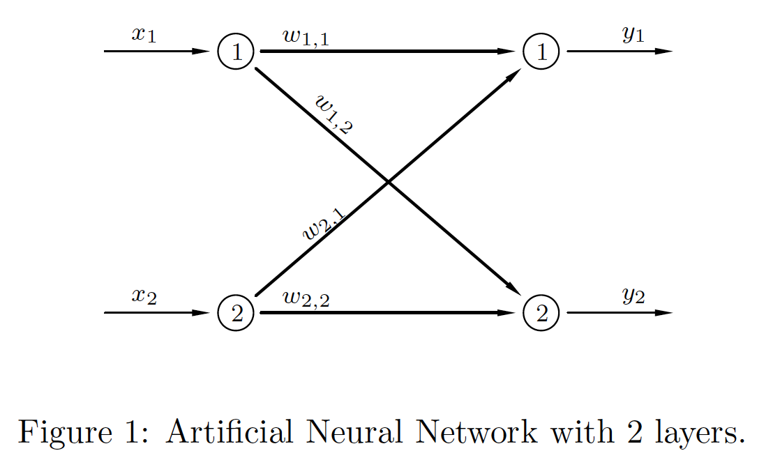
This is a simple 2-input/2-output shallow network (i.e. with no hidden layers).

|
This is a useful notation system... \begin{align*} \boldsymbol{a}_0 & = \boldsymbol{x}, \\ \boldsymbol{n}_1 & = \boldsymbol{W}_1^T\boldsymbol{a}_0+\boldsymbol{b}_1, \\ \boldsymbol{a}_1 & = \sigma_1(\boldsymbol{n}_1), \\ \boldsymbol{y} & = \boldsymbol{a}_1. \end{align*} Note that the weight matrices are square. |
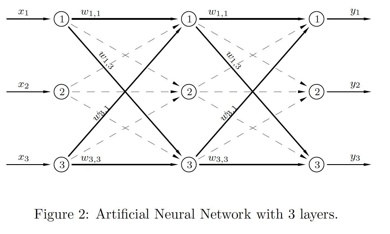
This is a 3-input/3-output network with one hidden layer.

|
The notation system is now easily adjusted... \begin{align*} \boldsymbol{a}_0 & = \boldsymbol{x}, \\ \boldsymbol{n}_1 & = \boldsymbol{W}_1^T\boldsymbol{a}_0+\boldsymbol{b}_1, \\ \boldsymbol{a}_1 & = \sigma_1(\boldsymbol{n}_1), \\ \boldsymbol{n}_2 & = \boldsymbol{W}_2^T\boldsymbol{a}_1+\boldsymbol{b}_2, \\ \boldsymbol{a}_2 & = \sigma_2(\boldsymbol{n}_2), \\ \boldsymbol{y} & = \boldsymbol{a}_2. \end{align*} The weight matrices are still square. |
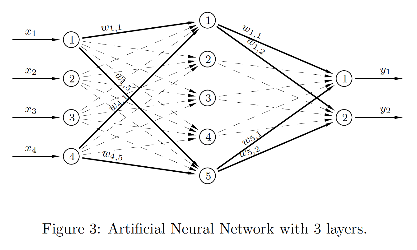
This is more general network with one hidden layer.

|
\begin{align*} \boldsymbol{a}_0 & = \boldsymbol{x}, \\ \boldsymbol{n}_1 & = \boldsymbol{W}_1^T\boldsymbol{a}_0+\boldsymbol{b}_1, \\ \boldsymbol{a}_1 & = \sigma_1(\boldsymbol{n}_1), \\ \boldsymbol{n}_2 & = \boldsymbol{W}_2^T\boldsymbol{a}_1+\boldsymbol{b}_2, \\ \boldsymbol{a}_2 & = \sigma_2(\boldsymbol{n}_2), \\ \boldsymbol{y} & = \boldsymbol{a}_2. \end{align*} In this general case the weight matrices are no longer square. |
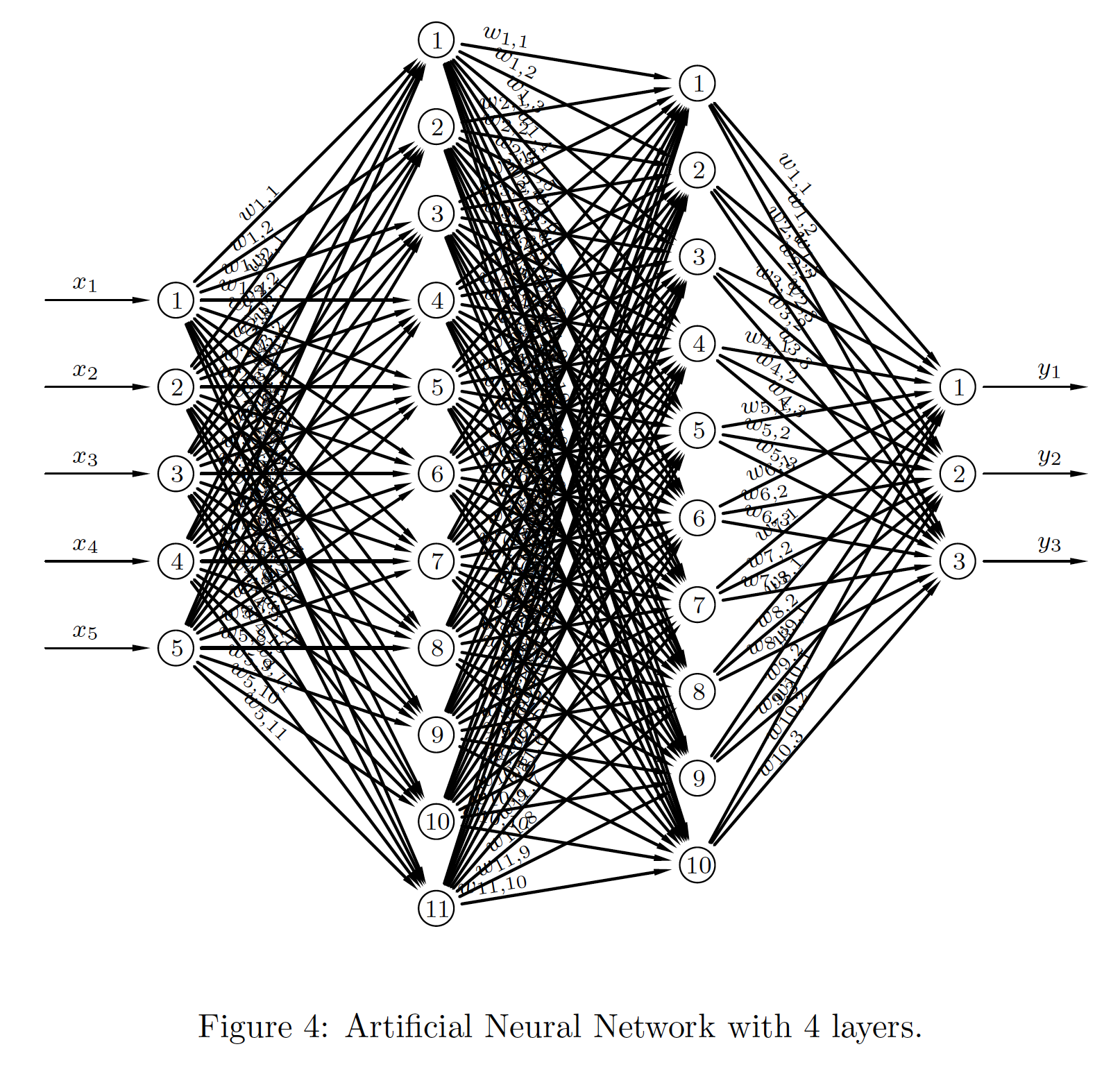
This is a more general network with two hidden layers.

|
\begin{align*} \boldsymbol{a}_0 & = \boldsymbol{x}, \\ \boldsymbol{n}_1 & = \boldsymbol{W}_1^T\boldsymbol{a}_0+\boldsymbol{b}_1, \\ \boldsymbol{a}_1 & = \sigma_1(\boldsymbol{n}_1), \\ \boldsymbol{n}_2 & = \boldsymbol{W}_2^T\boldsymbol{a}_1+\boldsymbol{b}_2, \\ \boldsymbol{a}_2 & = \sigma_2(\boldsymbol{n}_2), \\ \boldsymbol{n}_3 & = \boldsymbol{W}_3^T\boldsymbol{a}_2+\boldsymbol{b}_3, \\ \boldsymbol{a}_3 & = \sigma_3(\boldsymbol{n}_3), \\ \boldsymbol{y} & = \boldsymbol{a}_3. \end{align*} |
This assemblage of perceptons is called an artificial neural network. It is a very crude imitation of the neuronal connections in the brain.
Note that the weight matrix and bias vector have dimensions determined by the size of the layers they connect.
The architecture possibilities for a neural network are endless, and there are also variants on the basic scheme introduced above. These are,
Convolutional Neural Networks
Recurrent Neural Networks
... And lots more! It's a vibrant field!
The feed forward algortithm, for $L$ layers (not including the input layer) is
\begin{align*} & \boldsymbol{a}_0 = \boldsymbol{x}, \\ & \text{for } k = 1,2,\ldots,L, \\ &\qquad \boldsymbol{n}_k = \boldsymbol{W}_k^T\boldsymbol{a}_{k-1}+\boldsymbol{b}_k, \\ &\qquad \boldsymbol{a}_k = \sigma_k(\boldsymbol{n}_k), \\ &\boldsymbol{y} = \boldsymbol{a}_L. \end{align*}Activation Functions
The heaviside function is not differentiable - at least not in the usual and useful sense.
Other frequently used activation functions are the sigmoid (or logistic) function , and the ReLU - the Rectified Linear Unit.
$$ \mathrm{sigmoid}(x) = \frac{1}{1+\exp(-x)} \qquad\text{and}\qquad \mathrm{ReLU}(x) = \max\{0,x\} $$# here are some useful python function definitions of these
def sigmoid(x):
return 1/(1+np.exp(-x))
def ReLU(x):
return np.maximum(0,x)
xvals = np.arange(-5,5+0.1,0.1)
plt.plot(xvals, sigmoid(xvals), color='blue', label='sigmoid')
plt.plot(xvals, ReLU(xvals), color='red', label='ReLU')
plt.legend()
<matplotlib.legend.Legend at 0x7fcc382ee0b8>
The sigmoid we have seen before (logistic regression). The ReLU is new to us. Both of these are in frequent and common use in neural network development.
Here's an example of how to use them with our previous data $\boldsymbol{W}={\ \ \ 1\ \ 2 \choose-6\ \ 4}$ and $\boldsymbol{b}={1 \choose 2}$.
X = np.array([[1,-3]]).T
W = np.array([[1,2],[-6,4]])
b = np.array([[1,2]]).T
n = W.T @ X + b
ys = sigmoid(n)
yR = ReLU(n)
print(f'y = sigmoid(n) = \n{ys}\ny = ReLU(n) = \n{yR}, ')
y = sigmoid(n) =
[[9.99999998e-01]
 [3.35350130e-04]]
y = ReLU(n) =
[[20]
 [ 0]],
Review
We covered just enough, to make progress at pace. We looked at
- Perceptrons...
- weights, biases and various activation functions
- Vertically stacked fully connected perceptrons
- multi-layer perceptrons with hidded layers
- classification by partitioning the plane
This led us to artificial neural networks and will next take us on to deep learning.
There are two things to bring along with us:
In the above we knew the weights and biases - they gave us the classes.
We have only worked in two dimensions.
In practice our data lies in higher dimensional space. In such cases the data, bias and output vectors, and the weight matrices, are also high dimensional. Further, when we get our data set, we will not know the weights and biases in advance and we have to devise ways to machine learn them.