Artificial Neural Networks and Deep Learning

variationalform https://variationalform.github.io/

Just Enough: progress at pace

https://variationalform.github.io/

https://github.com/variationalform

Simon Shaw https://www.brunel.ac.uk/people/simon-shaw.

This work is licensed under CC BY-SA 4.0 (Attribution-ShareAlike 4.0 International) Visit http://creativecommons.org/licenses/by-sa/4.0/ to see the terms.

This document uses python

and also makes use of LaTeX

in Markdown

What this is about:

• Artificial Neural Networks

• Deep Learning

• MNIST digit recognition

As usual our emphasis will be on doing rather than proving: just enough: progress at pace

Assigned Reading

For this material you are recommended Chapter 3 of [UDL], then Chapter 3 of [NND], and Chapter 6 of [MLFCES].

• UDL: Understanding Deep Learning, by Simon J.D. Prince. PDF draft available here: https://udlbook.github.io/udlbook/
• NND: Neural Network Design by Martin T. Hagan, Howard B. Demuth, Mark Hudson Beale, Orlando De Jesús. https://hagan.okstate.edu/nnd.html and https://hagan.okstate.edu/NNDesign.pdf
• MLFCES: Machine Learning: A First Course for Engineers and Scientists, by Andreas Lindholm, Niklas Wahlström, Fredrik Lindsten, Thomas B. Schön. Cambridge University Press. http://smlbook.org.
• DL: Deep Learning, by Ian Goodfellow, Yoshua Bengio and Aaron Courville https://www.deeplearningbook.org

These can be accessed legally and without cost.

There are also these useful references for coding:

• PT: python: https://docs.python.org/3/tutorial
• NP: numpy: https://numpy.org/doc/stable/user/quickstart.html
• MPL: matplotlib: https://matplotlib.org

The [DL] book has rapidly become something of a classic - it's rich in content but might not be an easy introductory read: that will depend on the individual though.

Context

In the last section of this course we are going to take a look at the mathematical formulation of artificial neural networks.

We will be building on the feed forward algorithm we met in the section on perceptrons.

We know (or at least imagine) that, given the weights and biases, the network carves up the output space into compartments that can be used for classification.

But we need to start with training data, and use this to determine the weights and biases. We will cover the essentials of:

• cost, error, loss
• gradient descent
• hyperparameters
• back propagation
• activation functions

We start by looking at the data we are going to use: The MNIST data set of handwritten digits.

This will all be done manually - we wont use sklearn for this section

# our usual imports
import numpy as np
import matplotlib.pyplot as plt
import seaborn
import pandas
import matplotlib.pyplot as plt

MNIST Data Set of Handwritten Digits

The original source of these digitized images is here: http://yann.lecun.com/exdb/mnist/

This format isn't particularly easy to work with, so this site, https://pjreddie.com/projects/mnist-in-csv/, makes two CSV files available:

• MNIST_train.csv - $60,000$ handwritten digit images, for training
• MNIST_test.csv - $10,000$ handwritten digit images, for testing

Further, for testing and development it is useful to have small data sets, and so Rashid for his book Make Your Own Neural Network, at https://github.com/makeyourownneuralnetwork/makeyourownneuralnetwork, made these two smaller sets,

• MNIST_train_100.csv - $100$, for training
• MNIST_test_10.csv - $10$, for testing

This book was also used for these notes. Note that the test set here is not exhaustive in that not all labels are included. This means that you'll get errors below for the confusion mamtrix if you use this one.

There are also these (home made), for intermediate use:

• MNIST_train_1000.csv - $1000$, for training
• MNIST_test_100.csv - $100$, for testing

Let's get the data - you may need to need to grab it and unzip it from brightspace (or use binder).

We'll make it easy to choose which data set with a choice variable.

NOTE: MNIST_train.csv is not available in this git repo, or the binder environment because it is too big

choice = 2
if choice == 0:
  df_train = pandas.read_csv(r'./data/MNIST/MNIST_train.csv', header=None)
  df_test  = pandas.read_csv(r'./data/MNIST/MNIST_test.csv', header=None)
elif choice == 1:
  df_train = pandas.read_csv(r'./data/MNIST/MNIST_train_1000.csv', header=None)
  df_test  = pandas.read_csv(r'./data/MNIST/MNIST_test_100.csv', header=None)
elif choice == 2:
  df_train = pandas.read_csv(r'./data/MNIST/MNIST_train_100.csv', header=None)
  df_test  = pandas.read_csv(r'./data/MNIST/MNIST_test_100.csv', header=None)
else:
  df_train = pandas.read_csv(r'./data/MNIST/MNIST_train_100.csv', header=None)
  df_test  = pandas.read_csv(r'./data/MNIST/MNIST_test_10.csv', header=None)

# it will take a bit of work to see what these data files hold
df_train.head()

	0	1	2	3	4	5	6	7	8	9	...	775	776	777	778	779	780	781	782	783	784
0	5	0	0	0	0	0	0	0	0	0	...	0	0	0	0	0	0	0	0	0	0
1	0	0	0	0	0	0	0	0	0	0	...	0	0	0	0	0	0	0	0	0	0
2	4	0	0	0	0	0	0	0	0	0	...	0	0	0	0	0	0	0	0	0	0
3	1	0	0	0	0	0	0	0	0	0	...	0	0	0	0	0	0	0	0	0	0
4	9	0	0	0	0	0	0	0	0	0	...	0	0	0	0	0	0	0	0	0	0

5 rows × 785 columns

This doesn't look too promising ... but we'll get there.

The first column contains the labels. The remaining columns contain $28^2$ pixel values for the digitized image of the label.

Let's push on ...

# We assign the pixel values to X_train and X_test
X_train = df_train.iloc[:, 1:].values
X_test  = df_test.iloc[:, 1:].values
N_train = X_train.shape[0]
N_test  = X_test.shape[0]
print(f'N_train = {N_train}, N_test = {N_test}')

# And we assign the first column labels 0,1,2,...,9 to ... 
train_labels = df_train.iloc[:, 0].values
test_labels  = df_test.iloc[:, 0].values

print(X_train.shape)
print(X_test.shape)
print(train_labels.shape)
print(test_labels.shape)

N_train = 100, N_test = 100
(100, 784)
(100, 784)
(100,)
(100,)

Here are the first 10 labels in the training set...

print(train_labels[:9])

[5 0 4 1 9 2 1 3 1]

And now the first ten labels in the test set...

print(test_labels[:9])

[3 8 0 5 4 3 8 3 2]

We choose the third row (indexed as 2) in the training set to demonstrate

# Let's choose the third row (indexed as 2) 
row = 2
plt.imshow( X_train[row,:].reshape(28,28) , cmap='Greys', interpolation='None')
plt.title(f'Digitized Image With Label {train_labels[row]}')
print(f'There are 28x28 = {28*28} pixel values: 0,1,...,255')
print('0 is white, 255 is black 2,3,...,254 are grays')

There are 28x28 = 784 pixel values: 0,1,...,255
0 is white, 255 is black 2,3,...,254 are grays

# scale pixel values to [0,1] - this is recommended. 
X_train = X_train/255
X_test  = X_test/255
plt.imshow(X_train[row,:].reshape(28,28) , cmap='Greys', interpolation='None')

<matplotlib.image.AxesImage at 0x7fd220c4a6d8>

Our Neural Network

We want a neural network that will accept a digitized image as input

Each image yields $28^2=784$ inputs, one for each pixel value.

There are $10$ possible outputs - corresponding to the digits $\{0,1,2,3,4,5,6,7,8,9\}$.

Our network will have $10$ outputs. For a given input we want the output to be all zeros except for one which is unity. This non-zero will be in the position of the label.

So, if the label is $7$ then we want the output to be $(0,0,0,0,0,0,0,1,0,0)^T$. (Note the transpose - column vectors only.)

This is called one hot encoding. Let's set up the output (label) data for the training and the test sets.

# make every entry zero to begin with ...
y_train = np.zeros((10, N_train))
y_test = np.zeros((10, N_test))
print(f'Shape of: y_train = {y_train.shape}, y_test = {y_test.shape}')

Shape of: y_train = (10, 100), y_test = (10, 100)

One-Hot Encoding

We will one-hot encode the labels ready for implementation in a neural network. There are 10 possible output values corresponding to the labels $\{0,1,2,3,4,5,6,7,8,9\}$.

We want to use the train_labels and test_labels data from above to create y_train and y_test.

These will be matrices with each column having $10$ entries.

In y_train there will be as many columns as there are training data points (i.e. N_train). And in y_test there will be as many columns as there are test data points (i.e. N_test).

Each column contains zeros except for a single one in the position (0,1,2,...,9) corresponding to the label (0,1,2,...,9) for that column.

Above we saw that with choice = 2, the third data point in the training set had label $4$.

Hence the third column of y_train will be $(0,0,0,0,1,0,0,0,0,0)$.

We loop through the two data sets, grab each label in turn, and set that position equal to unity.

for k in range(N_train):
  label = train_labels[k]
  y_train[label,k] = 1

for k in range(N_test):
  label = test_labels[k]
  y_test[label,k] = 1

We can plot the sums to see how many of each label there are.

plt.bar(range(10),y_train.sum(axis=1), label='y train')
plt.bar(range(10),y_test.sum(axis=1), label='y test')
plt.legend()

<matplotlib.legend.Legend at 0x7fd1f08fba58>

And, because we like to always be checking our work, we can add up all the ones in each of these and make sure there are the same sumber as N_train and N_test.

# add up all the ones - across both dimensions
print(y_train.sum())
print(y_test.sum())

100.0
100.0

Recall that we've always insisted that our features vary along the columns, with our observations listed down the rows.

That's what we have done for X_train and X_test. Each row is an observation of a handwritten digit. Each column - pixel value - is a feature.

NOTE the term one hot is an electrical analogy wherein one terminal is considered hot and the other cold (i.e. on and off).

Our Neural Network Architecture

We have an input layer of $28^2=784$ nodes (neurons) accepting a pixel value per node, and an output layer of $10$ neurons capable of yielding a one-hot encoded output.

We'll choose two hidden layers with $500$ nodes on the first and $200$ on the second. These are all hyperparameters - we have to choose them and build them into our design. Once chosen they remain fixed.

We have already seen this type of network, along with the feed forward algorithm.

Here is an artificial neural network with two hidden layers.

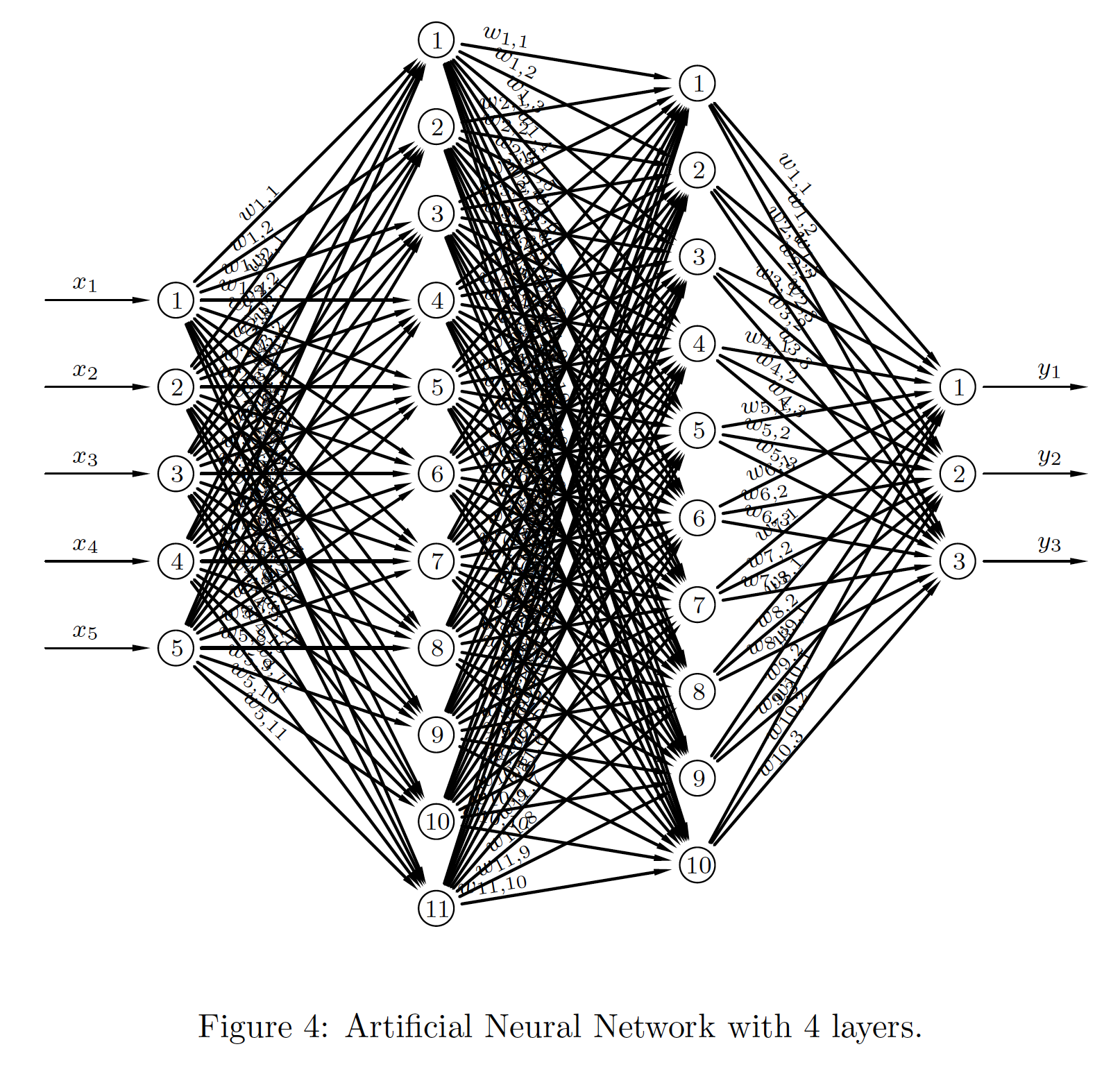
\begin{align*} \boldsymbol{a}_0 & = \boldsymbol{x}, \\ \boldsymbol{n}_1 & = \boldsymbol{W}_1^T\boldsymbol{a}_0+\boldsymbol{b}_1, \\ \boldsymbol{a}_1 & = \sigma_1(\boldsymbol{n}_1), \\ \boldsymbol{n}_2 & = \boldsymbol{W}_2^T\boldsymbol{a}_1+\boldsymbol{b}_2, \\ \boldsymbol{a}_2 & = \sigma_2(\boldsymbol{n}_2), \\ \boldsymbol{n}_3 & = \boldsymbol{W}_3^T\boldsymbol{a}_2+\boldsymbol{b}_3, \\ \boldsymbol{a}_3 & = \sigma_3(\boldsymbol{n}_3), \\ \boldsymbol{y} & = \boldsymbol{a}_3. \end{align*}

DEEP LEARNING

The addition of extra hidden layers between the input and output layers gives rise to the deep in DEEP LEARNING.

We'll see where the learning fits in shortly. We'lll need to learn the values of the weights and biases.

For the moment though we initialise our weights with fairly small random numbers, and set our biases to be zero. We'll use the training data to learn better values.

We initialise our network architecture along with the weights and biases as follows.

inn = 784  # number of nodes on input layer
h1n = 500  # number of nodes on first hidden layer
h2n = 200  # number of nodes on second hidden layer
onn = 10   # number of nodes on output layer

# weights and biases
W1 = 0.5 - np.random.rand(inn,h1n) # weights connecting input to first hidden
W2 = 0.5 - np.random.rand(h1n,h2n) # weights connecting first to second hidden
W3 = 0.5 - np.random.rand(h2n,onn) # weights connecting second hidden to output
b1 = np.zeros([h1n,1])             # bias on first hidden
b2 = np.zeros([h2n,1])             # bias on second hidden
b3 = np.zeros([onn,1])             # bias on output

print(f'W1 shape: {W1.shape}, W2 shape: {W2.shape}, W3 shape: {W3.shape}')
print(f'b1 shape: {b1.shape}, b2 shape: {b2.shape}, b3 shape: {b3.shape}')

W1 shape: (784, 500), W2 shape: (500, 200), W3 shape: (200, 10)
b1 shape: (500, 1), b2 shape: (200, 1), b3 shape: (10, 1)

The Feed Forward Algorithm

We have already seen this. The feed forward algortithm, for $L$ layers (not including the input layer) is,

\begin{align*} & \boldsymbol{a}_0 = \boldsymbol{x}, \\ & \text{for } k = 1,2,\ldots,L, \\ &\qquad \boldsymbol{n}_k = \boldsymbol{W}_k^T\boldsymbol{a}_{k-1}+\boldsymbol{b}_k, \\ &\qquad \boldsymbol{a}_k = \sigma_k(\boldsymbol{n}_k), \\ &\boldsymbol{y} = \boldsymbol{a}_L. \end{align*}

where $\sigma$ is the activation function. We have seen the Heaviside function for this, as well as the sigmoid and the ReLU.

We'll define them using python functions. We will also need their derivatives (and that's the main reason for not using the Heaviside step function - it isn't differentiable).

def sigmoid(x):
  return 1/(1+np.exp(-x))
def ReLU(x):
  return np.maximum(0,x)

def Diff_sigmoid(x):
  return sigmoid(x)*(1-sigmoid(x))
def Diff_ReLU(x):
  return np.heaviside(x,0)

# Let's plot them - just to remember what they look like
xvals = np.arange(-5,5+0.1,0.1)
plt.plot(xvals, sigmoid(xvals), color='blue', label='sigmoid')
xvals = np.arange(-5,2+0.1,0.1)
plt.plot(xvals, ReLU(xvals), color='red', label='ReLU')
plt.legend()

<matplotlib.legend.Legend at 0x7fd24129b358>

Feeding Forward - Forward Propagation

Here is a typical forward pass through the network. We choose a random integer, $k$ from $\{0,1,2,\ldots,N_{\mathrm{train}}\}$, and use that to select a training point at random. Then we apply the algorithm from above.

k = np.random.randint(0, X_train.shape[0])
a0 = X_train[k,:].T # a0 = X_train[[k],:].T #a0 = X_train[k,:].reshape(-1,1)
# feed into first hidden layer and activate
n1 = W1.T @ a0 + b1
a1 = sigmoid(n1)
# feed into second hidden layer and activate
n2 = W2.T @ a1 + b2
a2 = sigmoid(n2)
# feed into output layer and activate
n3 = W3.T @ a2 + b3
a3 = sigmoid(n3)
# produce output
y = a3

BUT THIS IS USELESS - the weights are random and the biases are zero. Whatever the input, the output will be random.

Learning - Artificial Intelligence (AI)

We want to use the training data to learn better values of the weights and biases.

By better we mean that given an input with label, say, $5$, the output should be $(0,0,0,0,0,1,0,0,0,0)^T$ - a one-hot encoding of the label corresponding to the input.

In practice our weights and biases may never be perfect, and so we might not get perfect one-hot outputs.

But we would be happy with, for example,

$$ (0.01,0.04,0.1,0.34,0.07,0.89,0.02,0.11,0.21,0.04)^T $$

Here $0.89\approx 1$ in the index $5$ position and the other values we treat as $\approx 0$.

If it works then we have created AI for digit recognition. This could be used for ANPR, handwriting, and it's not much of a conceptual step to move to digitized photos (face tagging) and voice (Alexa, Hi Siri, OK Google)...

No human needed...

But we need better weights and biases: we get them by setting up a cost and minimizing it.

Cost: Total Squared Error (TSE)

There are other choices, but we have seen this one before and so will use it.

For a given training point, indexed by $k$ say, we have two outputs. One we call the ground truth, and is stored in y_train. We will call this $\boldsymbol{t}_k$ for truth. It is perfectly one-hot encoded.

The other output is the prediction from the network which is given by $\boldsymbol{y}_k = \boldsymbol{a}_L$ in the feed-forward algorithm above. This will not be perfectly one-hot encoded but as we have seen above we can be happy with just picking the maximum value and using it as an approximation to a one-hot encoding.

We define the TSE cost as

$$ \mathcal{E}(\boldsymbol{W}_1,\boldsymbol{W}_2,\boldsymbol{W}_3, \boldsymbol{b}_1,\boldsymbol{b}_2,\boldsymbol{b}_3) = \sum_{k=1}^{N_{\mathrm{train}}} \mathscr{F}(\boldsymbol{t}_k,\boldsymbol{y}_k) $$$$\text{for the loss}\quad \mathscr{F}_k := \mathscr{F}(\boldsymbol{t}_k,\boldsymbol{y}_k) := \Vert\boldsymbol{t}_k-\boldsymbol{y}_k\Vert_2^2. $$

Normally we just write $\mathcal{E}$ for brevity, but we have to always bear in mind that it depends on all the weights and all the biases.

The Size of the Task

We want to choose all the weights and biases so as to minimize the error.

Recall the size of the weight matrices and bias vectors.

$$ \boldsymbol{W}_1 \in\mathbb{R}^{784\times500}, \ \boldsymbol{W}_2 \in\mathbb{R}^{500\times200}, \ \boldsymbol{W}_3 \in\mathbb{R}^{200\times10}, $$$$ \boldsymbol{b}_1 \in\mathbb{R}^{500}, \ \boldsymbol{b}_2 \in\mathbb{R}^{200}, \ \boldsymbol{b}_3 \in\mathbb{R}^{10}. $$

Wvals = W1.size + W2.size + W3.size
bvals = b1.size + b2.size + b3.size
print('Number of values to optimize = ', Wvals + bvals)

Number of values to optimize =  494710

There are nearly half a million values to optimize in the three full weight matrices, and the three bias vectors.

Gradient Descent

If you have ever studied multivariable calculus and looked at optimization problems you might have seen examples of how to optimize a function of two variables. For example,

$$ f(x,y) = 3\,{\mathrm{e}}^{-{\left(y+1\right)}^2-x^2}\,{\left(x-1\right)}^2 -\frac{{\mathrm{e}}^{-{\left(x+1\right)}^2-y^2}}{3} +{\mathrm{e}}^{-x^2-y^2}\,\left(10\,x^3-2\,x+10\,y^5\right). $$

You may remember that we need to calculate the gradient, $\nabla f$, set it to zero, $\nabla f=\boldsymbol{0}$, solve this for the optimal points, and then check the Hessian for the nature of these optimal points.

That isn't an option here. Instead the usual choice for minimizing the cost is Stochastic Gradient Descent.

Gradient Descent in Outline

The idea is to consider $\nabla f$ and note that this gives the direction in which $f$ increases most rapidly.

Therefore $-\nabla f$ tells us in which direction $f$ decreases most rapidly.

That's what we want - we want to get to the minimum. The bottom of the hill

We choose a point, $\boldsymbol{x}_0$ say, and then move to a new point by moving down the gradient. We then iterate:

\begin{align} \boldsymbol{x}_1 & = \boldsymbol{x}_0 - \alpha\nabla f(\boldsymbol{x}_0), \\ \boldsymbol{x}_2 & = \boldsymbol{x}_1 - \alpha\nabla f(\boldsymbol{x}_1), \\ \boldsymbol{x}_3 & = \boldsymbol{x}_2 - \alpha\nabla f(\boldsymbol{x}_2), \\ \vdots & \qquad\vdots\qquad \vdots \end{align}

Once we find a $k$ for which $\nabla f(\boldsymbol{x}_k)=\boldsymbol{0}$ (at least approximately) we stop - we'll be at a minimum (approximately). Note that it might not be a global minimum, and it could even be a saddle point.

Here, and in this context, $\alpha$ is called the learning rate. It is another hyperparameter. We choose it - it does not get learned by the algorithm.

Let's see some examples of how this might work in 2D.

 Gradient Descent Demonstrations - Global and Local Minima

Diagrams will not show in PDF version.

 Gradient Descent Demonstrations - Saddle Points

Diagrams will not show in PDF version.

 Stochastic Gradient (Descent?)

The Gradient Descent process described above is too computationally expensive for training big neural nets.

Ours has nearly half a million independent variables, but that is pretty modest by some standards.

This number of independent variables tells us how many gradient component directions there are.

Also N_train tells us how many loss terms there are in the cost function - these would need to be simultaneously minimized.

A variant, called Stochastic Gradient Descent, or SGD for short, is often used to save computer time and resources.

We'll use this in its simplest form (so-called mini-batch approaches exist) which is to just pick at random, and without replacement, one loss at a time and update with that.

Some people call this Stochastic Gradient instead of Stochastic Gradient Descent because it is not guaranteed that descent actually occurs at a given step.

Like so much of what we have done, there is so much more we could be saying on this topic.

The Calculus of Learning - part 1

We're going to just outline the main steps. A deep understanding of this is beyond our scope.

Consider the weight matrix connecting the second hidden layer to the output layer: $\boldsymbol{W}_3$ and let $w_{rc}$ denote the entry in row $r$ and column $c$. Also, consider $\boldsymbol{b}_3$ with $b_r$ in row $r$.

We choose a loss term at random - the $k$-th term say, $\mathscr{F}_k$ - and then an SGD update is then written like this

$$ w_{rc} \leftarrow w_{rc} -\alpha\frac{\partial\mathscr{F}_k}{\partial w_{rc}} \qquad\text{ and }\qquad b_{r} \leftarrow b_{r} -\alpha\frac{\partial\mathscr{F}_k}{\partial b_{r}} $$

where $\leftarrow$ means is replaced by. Now, $\mathscr{F}_k = \Vert\boldsymbol{t}_k-\boldsymbol{y}_k\Vert_2^2$ and so, concentrating on the weights,

$$ \frac{\partial\mathscr{F}_k}{\partial w_{rc}} = \frac{\partial}{\partial w_{rc}} \Vert\boldsymbol{t}_k-\boldsymbol{y}_k\Vert_2^2 = \frac{\partial}{\partial w_{rc}} \sum_{\ell=1}^{10} (t_{\ell k}- y_{\ell k})^2. $$

In this $\boldsymbol{t}_k$ is a constant, so we need to think about $y_{\ell k}$.

The Calculus of Learning - part 2

We recall the forward prop algorithm:

\begin{align*} \boldsymbol{a}_0 & = \boldsymbol{x}, \\ \boldsymbol{n}_1 & = \boldsymbol{W}_1^T\boldsymbol{a}_0+\boldsymbol{b}_1, \\ \boldsymbol{a}_1 & = \sigma_1(\boldsymbol{n}_1), \\ \boldsymbol{n}_2 & = \boldsymbol{W}_2^T\boldsymbol{a}_1+\boldsymbol{b}_2, \\ \boldsymbol{a}_2 & = \sigma_2(\boldsymbol{n}_2), \\ \boldsymbol{n}_3 & = \boldsymbol{W}_3^T\boldsymbol{a}_2+\boldsymbol{b}_3, \\ \boldsymbol{a}_3 & = \sigma_3(\boldsymbol{n}_3), \\ \boldsymbol{y} & = \boldsymbol{a}_3. \end{align*}

In this it is the $k$-th component of $\boldsymbol{y} = \boldsymbol{a}_3$ that we are dealing with.

The Calculus of Learning - part 3

So, we look at the $k$-th component and calculate...

$$ \frac{\partial\mathscr{F}_k}{\partial w_{rc}} = \frac{\partial}{\partial w_{rc}} \sum_{\ell=1}^{10} (t_{\ell k}- y_{\ell k})^2 = -2\sum_{\ell=1}^{10} (t_{\ell k}- y_{\ell k}) \frac{\partial y_{\ell k}}{\partial w_{rc}} $$

But (with $L=10$ outputs and $H=200$ neurons on the second hidden layer), and $\boldsymbol{a}_2 = (a_1, a_2, \ldots)^T$,

$$ y_{\ell k} = \sigma(n_{\ell}) \quad\text{for}\quad n_{\ell} = \sum_{h=1}^{H} w_{h\ell}a_h + b_\ell \quad\text{ and }\quad \frac{\partial y_{\ell k}}{\partial w_{rc}} = \sigma'(n_{\ell}) \frac{\partial n_{\ell}}{\partial w_{rc}} $$

with $\boldsymbol{n}_{3k} = (n_1, n_2, \ldots)^T$. It follows that

$$ \frac{\partial n_{\ell k}}{\partial w_{rc}} = \frac{\partial}{\partial w_{rc}}\sum_{h=1}^{H} w_{h\ell}a_h + b_\ell \quad\text{ hence }\quad \frac{\partial n_{\ell k}}{\partial w_{rc}} = a_r\delta_{c\ell} $$

where $\delta_{ij} = 1$ if $i=j$ and $\delta_{ij} = 0$ otherwise (called the Kronecker delta).

The Calculus of Learning - part 4

Putting this together we then get, first,

$$ \frac{\partial y_{\ell k}}{\partial w_{rc}} = \sigma'(n_{\ell k}) \frac{\partial n_{\ell k}}{\partial w_{rc}} = \sigma'(n_{\ell k}) a_r\delta_{c\ell}. $$

Therefore, for $e_{\ell k} = t_{\ell k}- y_{\ell k}$,

$$ \frac{\partial\mathscr{F}_k}{\partial w_{rc}} = -2\sum_{\ell=1}^{10} (t_{\ell k}- y_{\ell k}) \sigma'(n_{\ell k}) a_r\delta_{c\ell} = -2\sum_{\ell=1}^{10} e_{\ell k} \sigma'(n_{\ell k}) a_r\delta_{c\ell} $$

Let $\displaystyle\frac{\partial\mathscr{F}_k}{\partial \boldsymbol{W}_3}$ be the matrix with $\displaystyle\frac{\partial\mathscr{F}_k}{\partial w_{rc}}$ in row $r$ and column $c$. Then, after some manipulations, it can be shown that,

$$ \frac{\partial\mathscr{F}_k}{\partial \boldsymbol{W}_3} = \boldsymbol{a}_2 \boldsymbol{S}_3^T \text{ for } \boldsymbol{S}_3 = -2 \boldsymbol{A}_3\boldsymbol{e}_k \text{ and } \boldsymbol{A}_3 = \left(\begin{array}{llll} \sigma'(n_1) & 0 & 0 & \cdots \\ 0 & \sigma'(n_2) & 0 & \cdots \\ 0 & 0 & \sigma'(n_3) & \cdots \\ \vdots & \vdots & \vdots & \ddots \end{array}\right). $$

The Calculus of Learning - part 5

With similar manipulations it can also be shown that $\displaystyle\frac{\partial\mathscr{F}_k}{\partial \boldsymbol{b}_3} = \boldsymbol{S}$.

The gradient updates from earlier,

$$ w_{rc} \leftarrow w_{rc} -\alpha\frac{\partial\mathscr{F}_k}{\partial w_{rc}} \qquad\text{ and }\qquad b_{r} \leftarrow w_{r} -\alpha\frac{\partial\mathscr{F}_k}{\partial b_{r}} $$

can now be written in explicit and computable form as,

$$ \boldsymbol{W}_3 \leftarrow \boldsymbol{W}_3 - \alpha \boldsymbol{a}_2 \boldsymbol{S}_3^T \qquad\text{ and }\qquad \boldsymbol{b}_3 \leftarrow \boldsymbol{b}_3 - \alpha \boldsymbol{S}_3 $$

These tell us how to update the weights and biases at the output end of the network.

But what about $\boldsymbol{W}_2$, $\boldsymbol{b}_2$ and $\boldsymbol{W}_1$, $\boldsymbol{b}_1$?

The Calculus of Learning - part 6

To update the weights and biases further down towards the start of the network we need

$$ w_{rc} \leftarrow w_{rc} -\alpha\frac{\partial\mathscr{F}_k}{\partial w_{rc}} \qquad\text{ and }\qquad b_{r} \leftarrow w_{r} -\alpha\frac{\partial\mathscr{F}_k}{\partial b_{r}} $$

where $w_{rc}$ and $b_r$ now refer to $\boldsymbol{W}_2$, $\boldsymbol{b}_2$ first, and then to $\boldsymbol{W}_1$, $\boldsymbol{b}_1$.

We could attempt a direct calculation, as above, but this would get quite involved as the number of layers increases. Instead we use the back propagation formula:

$$ \boldsymbol{S}_{i-1}=\boldsymbol{A}_{i-1}\boldsymbol{W}_i\boldsymbol{S}_i $$

which is applied for $i=L, L-1, \ldots, 2$.

The derivation of this is quite involved.

The Calculus of Learning - part 7

We consider two consecutive layers, $i-1$ and $i$, connected with the weights in $\boldsymbol{W}_i$ and with biases $\boldsymbol{b}_i$ added on layer $i$. Assume there are $H$ nodes on layer $i-1$ and $L$ on layer $i$. We use hats to denote quantities on layer $i-1$, and then the key formulae are,

$$ n_c = \sum_{\ell=1}^H w_{\ell c} \hat{a}_\ell + b_c, \quad \hat{\boldsymbol{a}} = \sigma_{i-1}(\hat{\boldsymbol{n}}) \quad\text{ and }\quad \boldsymbol{a} = \sigma_i(\boldsymbol{n}). $$

Then (and similarly for the biases),

$$ \boldsymbol{W} \leftarrow \boldsymbol{W} - \alpha \frac{\partial\mathscr{F}}{\partial w_{rc}} \quad\text{ uses }\quad \frac{\partial\mathscr{F}}{\partial w_{rc}} = \frac{\partial\mathscr{F}}{\partial n_{c}} \frac{\partial n_c}{\partial w_{rc}} $$$$ \text{with } \frac{\partial n_c}{\partial w_{rc}} = \frac{\partial }{\partial w_{rc}} \sum_{\ell=1}^H w_{\ell c} \hat{a}_\ell + b_c = \hat{a}_r \Longrightarrow \frac{\partial\mathscr{F}}{\partial w_{rc}} = \hat{a}_r S_c \text{ with } \boldsymbol{S} = \left(\begin{array}{c} \partial\mathscr{F}/\partial n_1 \\ \partial\mathscr{F}/\partial n_2 \\ \partial\mathscr{F}/\partial n_3 \\ \vdots \end{array}\right) $$

The Calculus of Learning - part 8

We can conclude from this that

$$ \frac{\partial\mathscr{F}}{\partial\boldsymbol{W}_i} = \hat{\boldsymbol{a}}\boldsymbol{S}^T \quad\text{ and } \frac{\partial\mathscr{F}}{\partial\boldsymbol{b}_i} = \boldsymbol{S} $$

just as earlier at the output layer.

A key step is now to introduce the Jacobian Matrix

$$ \frac{\partial\boldsymbol{n}}{\partial\hat{\boldsymbol{n}}} = \left(\begin{array}{cccc} \partial n_1/\partial\hat{n}_1 & \partial n_1/\partial\hat{n}_2 & \partial n_1/\partial\hat{n}_3 & \cdots \\ \partial n_2/\partial\hat{n}_1 & \partial n_2/\partial\hat{n}_2 & \partial n_2/\partial\hat{n}_3 & \cdots \\ \partial n_3/\partial\hat{n}_1 & \partial n_3/\partial\hat{n}_2 & \partial n_3/\partial\hat{n}_3 & \cdots \\ \vdots & \vdots & \vdots & \ddots \end{array}\right) $$

and then use $\hat{\boldsymbol{a}} = \hat{\sigma}(\hat{\boldsymbol{n}})$ to calculate

$$ \frac{\partial n_c}{\partial\hat{n}_r} = \frac{\partial }{\partial\hat{n}_r} \sum_{\ell=1}^H w_{\ell c} \hat{a}_\ell + b_c = w_{rc}\frac{\partial\hat{a}_r}{\partial\hat{n}_r} = w_{rc}\hat{\sigma}'(\hat{n}_r). $$

The Calculus of Learning - part 9

It follows that

$$ \frac{\partial\boldsymbol{n}}{\partial\hat{\boldsymbol{n}}} = \boldsymbol{W}^T\hat{\boldsymbol{A}} \quad\text{ for }\quad \hat{\boldsymbol{A}} = \left(\begin{array}{llll} \hat{\sigma}'(\hat{n}_1) & 0 & 0 & \cdots \\ 0 & \hat{\sigma}'(\hat{n}_2) & 0 & \cdots \\ 0 & 0 & \hat{\sigma}'(\hat{n}_3) & \cdots \\ \vdots & \vdots & \vdots & \ddots \end{array}\right). $$

From above we define $\hat{\boldsymbol{S}}$ analogously to $\boldsymbol{S}$ as

$$ \hat{\boldsymbol{S}} = \left(\begin{array}{c} \partial\mathscr{F}/\partial \hat{n}_1 \\ \partial\mathscr{F}/\partial \hat{n}_2 \\ \partial\mathscr{F}/\partial \hat{n}_3 \\ \vdots \end{array}\right) \quad\text{ then }\quad \hat{S}_r = \frac{\partial\mathscr{F}}{\partial\hat{n}_r} = \sum_\ell\frac{\partial n_\ell}{\partial\hat{n}_r}\frac{\partial\mathscr{F}}{\partial n_\ell} = \sum_\ell\frac{\partial n_\ell}{\partial\hat{n}_r}S_\ell $$$$ \text{and so } \hat{\boldsymbol{S}} = \left(\frac{\partial\boldsymbol{n}}{\partial\hat{\boldsymbol{n}}}\right)^T\boldsymbol{S} = \left(\boldsymbol{W}^T\hat{\boldsymbol{A}}\right)^T\boldsymbol{S} = \hat{\boldsymbol{A}}\boldsymbol{W}\boldsymbol{S} \text{ because } \hat{\boldsymbol{A}}=\hat{\boldsymbol{A}}^T. $$

The Calculus of Learning - part 10

Layer-by-layer this recursion is $\boldsymbol{S}_{i-1}=\boldsymbol{A}_{i-1}\boldsymbol{W}_i\boldsymbol{S}_i$ and is called back propagation.

From above we have

$$ \frac{\partial\mathscr{F}}{\partial\boldsymbol{W}_i} = \boldsymbol{a}_{i-1}\boldsymbol{S}_i^T \quad\text{ and } \frac{\partial\mathscr{F}}{\partial\boldsymbol{b}_i} = \boldsymbol{S}_i $$

We have $\boldsymbol{S}_L = -2\boldsymbol{A}_i\boldsymbol{e}$ at the output layer, and we can compute $\boldsymbol{S}_{L-1}$, $\boldsymbol{S}_{L-2}$, $\boldsymbol{S}_{L-3}, \ldots$, recursively from the SAWS backprop recursion $\boldsymbol{S}_{i-1}=\boldsymbol{A}_{i-1}\boldsymbol{W}_i\boldsymbol{S}_i$

We now have eveything we need...

The Forward and Backward Propagation ('backprop') Algorithm - Learning from Data

\begin{align*} \begin{array}{rl} \text{forward} &\text{prop} \\\ \\ \boldsymbol{a}_0 & = \boldsymbol{x}, \\ \boldsymbol{n}_1 & = \boldsymbol{W}_1^T\boldsymbol{a}_0+\boldsymbol{b}_1, \\ \boldsymbol{a}_1 & = \sigma_1(\boldsymbol{n}_1), \\ \boldsymbol{n}_2 & = \boldsymbol{W}_2^T\boldsymbol{a}_1+\boldsymbol{b}_2, \\ \boldsymbol{a}_2 & = \sigma_2(\boldsymbol{n}_2), \\ \boldsymbol{n}_3 & = \boldsymbol{W}_3^T\boldsymbol{a}_2+\boldsymbol{b}_3, \\ \boldsymbol{a}_3 & = \sigma_3(\boldsymbol{n}_3), \\ \boldsymbol{y} & = \boldsymbol{a}_3. \end{array} \qquad &\qquad \begin{array}{rl} \text{back} &\text{prop} \\\ \\ \boldsymbol{e}_k & = \boldsymbol{t}_k-\boldsymbol{y}_k, \\ \boldsymbol{S}_3 & = -2\boldsymbol{A}_3\boldsymbol{e}_k, \\ \boldsymbol{W}_3 & \leftarrow \boldsymbol{W}_3 - \alpha \boldsymbol{a}_2 \boldsymbol{S}_3^T \text{ and } \boldsymbol{b}_3 \leftarrow \boldsymbol{b}_3 - \alpha \boldsymbol{S}_3 \\ \boldsymbol{S}_2 & = \boldsymbol{A}_2\boldsymbol{W}_3\boldsymbol{S}_3 \\ \boldsymbol{W}_2 & \leftarrow \boldsymbol{W}_2 - \alpha \boldsymbol{a}_1 \boldsymbol{S}_2^T \text{ and } \boldsymbol{b}_2 \leftarrow \boldsymbol{b}_2 - \alpha \boldsymbol{S}_2 \\ \boldsymbol{S}_1 & = \boldsymbol{A}_1\boldsymbol{W}_2\boldsymbol{S}_2 \\ \boldsymbol{W}_1 & \leftarrow \boldsymbol{W}_1 - \alpha \boldsymbol{a}_0 \boldsymbol{S}_1^T \text{ and } \boldsymbol{b}_1 \leftarrow \boldsymbol{b}_1 - \alpha \boldsymbol{S}_1 \end{array} \end{align*}

 Our Neural Network - training and testing

Here is the basic implementation algortithm for learning and testing

• Choose hyperparameters such as learning rate $\alpha$ and network architecture.

• Choose a positive integer $N_{\mathrm{epochs}}$ as the number of epochs to use in training. An epoch is a single loop through the whole training set, updating weights and biases for each data point.

• For each epoch, loop through the training points by choosing integers $k$ at random from $\{0,1,2,\ldots,N_{\mathrm{train}}-1\}$ without replacement (in code the indices start at zero).

  • Forward prop that training data point and calculate the error $\boldsymbol{e}_k = \boldsymbol{t}_k - \boldsymbol{y}_k$

  • Use the error to initiate the backprop and gradient descent updates.

  • Repeat for the next $k$

• At the end of each epoch update the cost $\mathcal{E}$ for later plotting.

• At the end of training, run the test data through one point at a time, and use the approximate one-hot encoding in the outputs $\boldsymbol{y}$ to assess the accuracy of the network.

The random selection is done without replacement. We use

ransel = np.random.permutation(N_train)

which gives us an array containing a random permutation of the indices in [0,1,2,...,N_train-1].

Here's the code...

# select a learning rate for SGD
alpha = 0.3
# loop through this many epochs
N_ep = 50
# initialise the TSE cost
TSEcost = np.zeros([N_ep,1])

We train by looping N_ep times through the training set.

Each training set loop randomly selects a loss term in the total cost with which to learn (update) new values for the weights and biases.

In the slides view the next cell will not fully display - it is too long.

for ep in range(N_ep): 
  ransel = np.random.permutation(N_train)
  for k in range(N_train):
    # select a random without replacement
    j = ransel[k]
    # forward prop
    a0 = X_train[[j],:].T 
    n1 = W1.T @ a0 + b1
    a1 = sigmoid(n1)
    n2 = W2.T @ a1 + b2
    a2 = sigmoid(n2)
    n3 = W3.T @ a2 + b3
    a3 = sigmoid(n3)
    y = a3
    # backprop and update
    error = y_train[:,[j]] - y
    A3 = np.diagflat(Diff_sigmoid(n3))
    A2 = np.diagflat(Diff_sigmoid(n2))
    A1 = np.diagflat(Diff_sigmoid(n1))
    S3 = -2*A3@error
    S2 = A2@W3@S3
    S1 = A1@W2@S2

    W3 = W3 - alpha * a2@S3.T
    W2 = W2 - alpha * a1@S2.T
    W1 = W1 - alpha * a0@S1.T

    b3 = b3 - alpha * S3
    b2 = b2 - alpha * S2
    b1 = b1 - alpha * S1

  # update cost - loop through training set
  for j in range(N_train):
    a0 = X_train[[j],:].T
    n1 = W1.T @ a0 + b1
    a1 = sigmoid(n1)
    n2 = W2.T @ a1 + b2
    a2 = sigmoid(n2)
    n3 = W3.T @ a2 + b3
    a3 = sigmoid(n3)
    y = a3
    error = y_train[:,[j]] - y
    TSEcost[ep] += (error * error).sum()

It is usual to plot the cost against epochs. We want to see the cost reduce to zero, or at least near-zero. If it doesn't then our training is not effective and we would consider adjusting the hyperparameters. These are:

• network architecture: number of hidden layers, nodes per layer
• learning rate
• number of epochs

plt.plot(range(N_ep), TSEcost)
plt.xlabel('epoch'); plt.ylabel('cost')

Text(0, 0.5, 'cost')

 Testing

Once it is trained we want to test the network's predictions on unseen data. We'll store all the predictions for a confusion matrix, and also create scorecards.

# test - create a matrix to hold the predictions
y_pred = np.zeros((10, X_test.shape[0]))
print(f'Shape of y_test = {y_test.shape}')
print(f'Shape of y_pred = {y_pred.shape}')

# create scorecards...
success = np.zeros(10)
failure = np.zeros(10)

Shape of y_test = (10, 100)
Shape of y_pred = (10, 100)

for k in range(N_test):
  # forward prop
  a0 = X_test[[k],:].T   # a0 = X_test[k,:].reshape(-1,1)
  n1 = W1.T @ a0 + b1
  a1 = sigmoid(n1)
  n2 = W2.T @ a1 + b2
  a2 = sigmoid(n2)
  n3 = W3.T @ a2 + b3
  a3 = sigmoid(n3)
  y_pred[:,[k]] = a3  
  if np.argmax(a3) == test_labels[k]:
    success[test_labels[k]] += 1
  else:
    failure[test_labels[k]] += 1

print(success)
print(failure)

[10. 10.  8.  9.  7.  2.  9.  6.  5.  6.]
[0. 0. 2. 1. 3. 8. 1. 4. 5. 4.]

Confusion Matrices

We have seen these before. We need to determine the positions of the maximum entries in the computed approximate one-hot encodings.

y_test_cm = np.zeros(N_test)
y_pred_cm = np.zeros(N_test)
test_indx_max = np.argmax(y_test, axis=0)
pred_indx_max = np.argmax(y_pred, axis=0)
for k in range(N_test):
  y_test_cm[k] = test_indx_max[k]
  y_pred_cm[k] = pred_indx_max[k]

from sklearn.metrics import confusion_matrix, accuracy_score
cm = confusion_matrix(y_test_cm, y_pred_cm)
print("Confusion Matrix:")
print(cm)
accsc = accuracy_score(y_test_cm,y_pred_cm)
print("Accuracy:", accsc)

Confusion Matrix:
[[10  0  0  0  0  0  0  0  0  0]
 [ 0 10  0  0  0  0  0  0  0  0]
 [ 0  1  8  0  0  0  1  0  0  0]
 [ 1  0  0  9  0  0  0  0  0  0]
 [ 0  0  0  0  7  1  0  0  0  2]
 [ 1  0  0  3  2  2  1  1  0  0]
 [ 0  0  0  0  0  0  9  0  0  1]
 [ 0  0  0  0  0  0  0  6  1  3]
 [ 0  2  0  1  0  0  1  0  5  1]
 [ 0  1  0  1  2  0  0  0  0  6]]
Accuracy: 0.72

from sklearn.metrics import ConfusionMatrixDisplay
cmplot = ConfusionMatrixDisplay(cm, display_labels=range(10))
#plt.figure(figsize=(15, 15))
#cmplot.plot()
fig, ax = plt.subplots(figsize=(6,6))
cmplot.plot(ax=ax);

Review

We got modest accuracy. Can you do better?

You can obtain the MNIST data from

https://variationalform.github.io/downloads/MNIST.zip

There are some handwritten notes that expand further on the maths of backprop. They are here:

https://variationalform.github.io/downloads/Backprop.pdf

We covered just enough, to make progress at pace. We looked at

• neural network Architecture
• training: cost, and backprop
• testing and evaluation

There is much much more - as usual.

Let's finish with a few observations.

Activation Functions and Cost

We used the sigmoid rather than the Heaviside because we needed its derivative in the backprop algorithm. It also gives us output values between zero and one which is useful for the approximate one-hot encoding.

However, we could have used the ReLU on the hidden layers. You can try this - you just need to alter those activations in the traiing and testing forward prop, and also in the backprop.

There is also a cost function that can be described as a cross entropy. This is used with a softmax activation on the final layer. We wont cover that here, but be aware that this approach is often claimed to be superior for deep learning classification tasks.

Deep Learning can also be used for regression.

Power Consumption

There are some live discussions out there regarding the carbon footprint of intensive computation. Machine Learning and AI in particular need a lot of such power.

It is worth giving it some thought.

Here are the results of a crude experiment

On a Mac, in the Terminal app, this command gives details of the battery.

system_profiler SPPowerDataType

With a fully charged battery, the charger was disconnected, the display dimmed, and this notebook was run five times up to the point where the cost is plotted against epochs.

The command above reported $6439\,\mathrm{mAh}$ at the start, and $6132\,\mathrm{mAh}$ after the five runs, and also reported a $12.5\,\mathrm{V}$ battery.

This was for 50 epochs, with a [784, 500, 200, 10] architecture.

Let's compare this energy cost to having a standard $28\,\mathrm{W}$ light bulb switched on.

print( (6439 - 6132)/5, ' mAh per training cycle')
print( (6439 - 6132)/5/1000, ' Ah per training cycle')
print( 12.5*(6439 - 6132)/5/1000, ' Wh per training cycle')
print( 28 / (12.5*(6439 - 6132)/5/1000), ' training cycles for 1 hour of a 28 watt bulb')

61.4  mAh per training cycle
0.061399999999999996  Ah per training cycle
0.7675  Wh per training cycle
36.48208469055375  training cycles for 1 hour of a 28 watt bulb

Comments? Thoughts? What about those big server farms?

The Tensorflow Playground

Tensorflow is a widely used deep learning library. This web page http://playground.tensorflow.org allows you to configure your own neural net, play with the hyper parameters, and see the effect for various classification problems.

PyTorch is similarly widely used. There are also others but these are ones we seem to hear most about.

Deep Learning in a few lines

The code that follows came from https://twitter.com/svpino/status/1582703127651721217 on 21 Oct 2023.

It shows that you can implement deep learning with just a few lines if the problem and data are simple enough.

This code learns logic gates. You can read about the Exclusive OR in particular in the [DL] book, Chapter 6.

This code might not dosplay properly in the slides medium - it's too long.

import numpy as np

def sigmoid(x):
  return 1 / (1+np.exp(-x))

def neural_network(X,y):
    learning_rate = 0.1
    W1 = np.random.rand(2,4)
    W2 = np.random.rand(4,1)
    
    for epoch in range(1000):
        layer1 = sigmoid(np.dot(X, W1))
        output = sigmoid(np.dot(layer1, W2))
        error = y-output
        delta2 = 2 * error * (output * (1 - output))
        delta1 = delta2.dot(W2.T) * (layer1 * (1 - layer1))
        W2 += learning_rate * layer1.T.dot(delta2)
        W1 += learning_rate * X.T.dot(delta1)
    
    return np.round(output).flatten()

X = np.array([[0,0],[0,1],[1,0],[1,1]])

print(  "OR", neural_network( X, np.array([[0,1,1,1]]).T ) )
print( "AND", neural_network( X, np.array([[0,0,0,1]]).T ) )
print( "XOR", neural_network( X, np.array([[0,1,1,0]]).T ) )
print("NAND", neural_network( X, np.array([[1,1,1,0]]).T ) )
print( "NOR", neural_network( X, np.array([[1,0,0,0]]).T ) )

OR [1. 1. 1. 1.]
AND [0. 0. 0. 1.]
XOR [0. 1. 1. 1.]
NAND [1. 1. 1. 0.]
NOR [1. 0. 0. 0.]